空調機シミュレーションにおける Amazon Timestream 活用【後半】
こんにちは、NRIデジタルの島です。
空調機シミュレーションにおける Amazon Timestream 活用【前半】では、Timestreamの概要、Timestream検証構成・構築、データの書き込みについて紹介しました。
【後半】は、Timestreamのデータ可視化、Timestreamの機能(補間関数・スケジュールドクエリ)、考察についてです。
時系列データの可視化
データの書き込みが完了したので、そのデータを可視化しようと思います。
※可視化にはシングルメジャーレコードのデータモデルを使用します
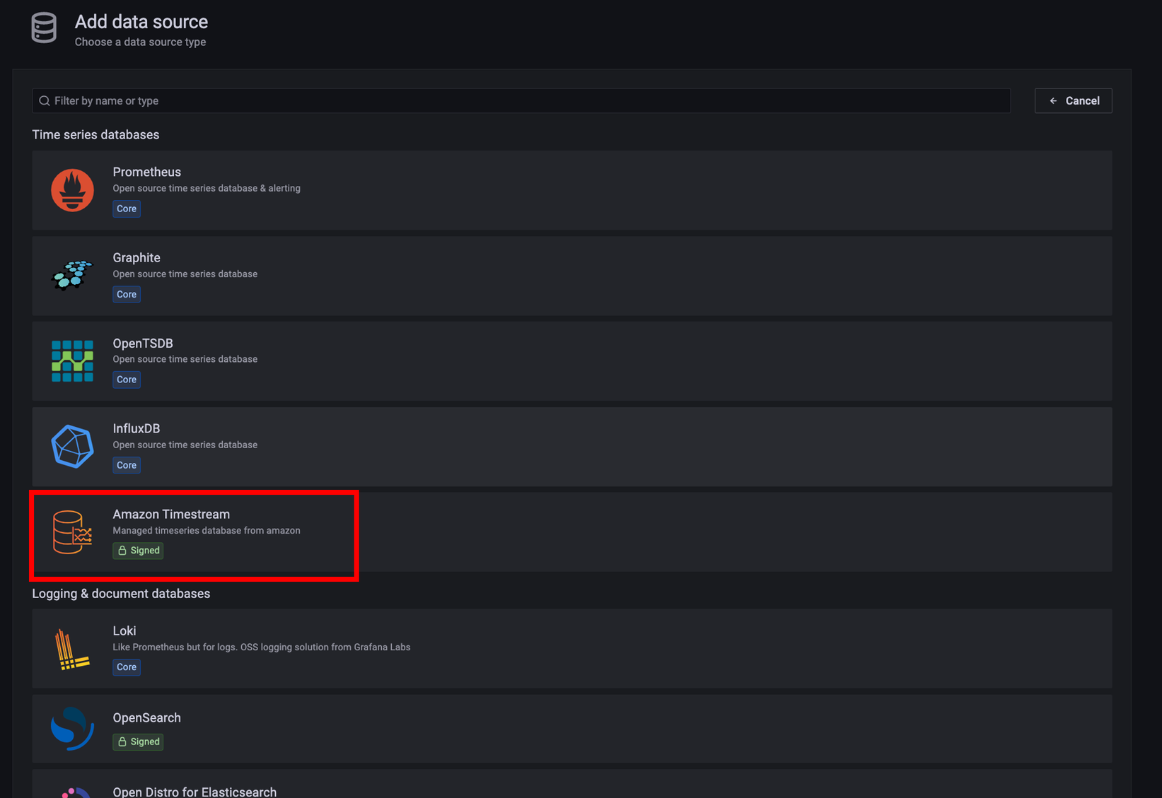
可視化ツールには前述の通りAMGでGrafanaを使用します。
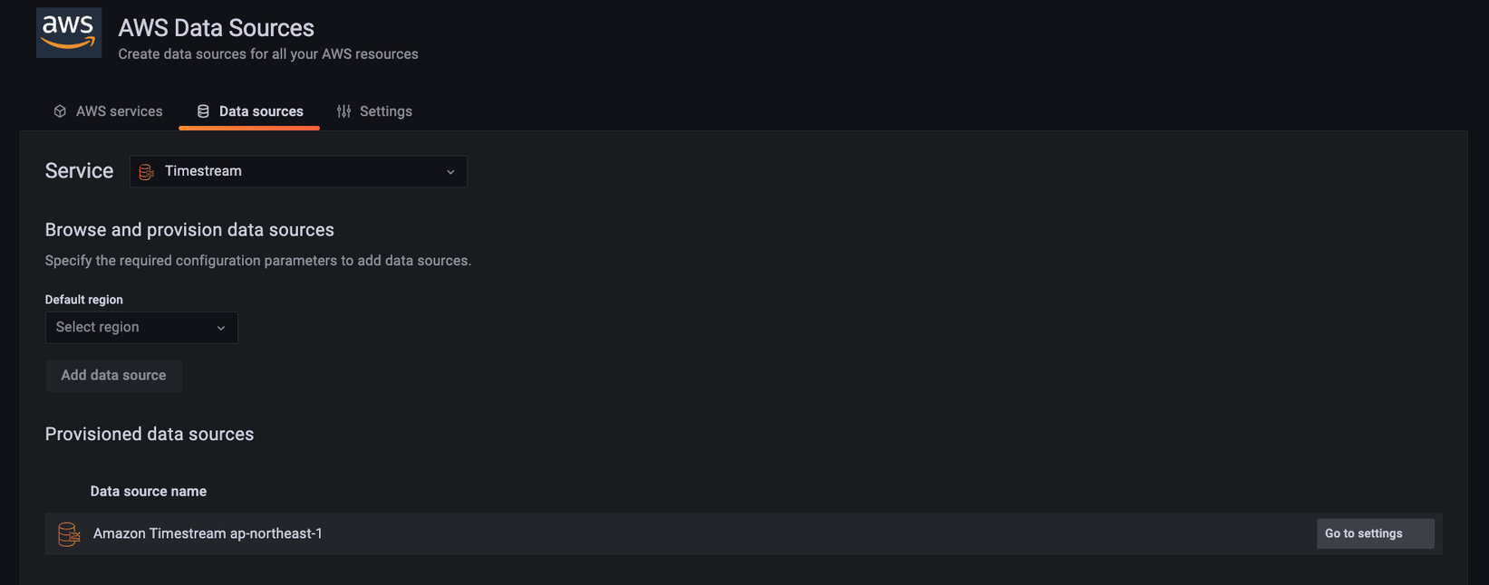
GrafanaのデータソースにTimestreamを設定します。
ダッシュボードを作成し、クエリを記述し可視化していきます。
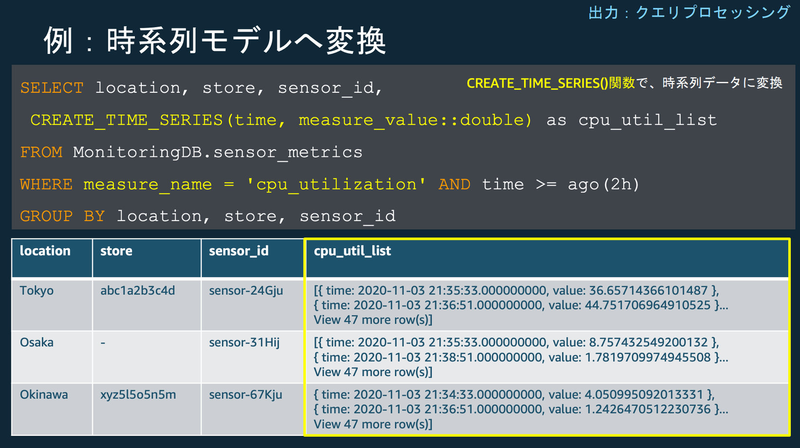
クエリに時系列モデルへの変換関数を指定することで簡単に時系列データの可視化が可能です。
どのようなクエリや関数が使用できるかについては、以下クエリリファレンスをご参照ください。
Query language reference – Amazon Timestream
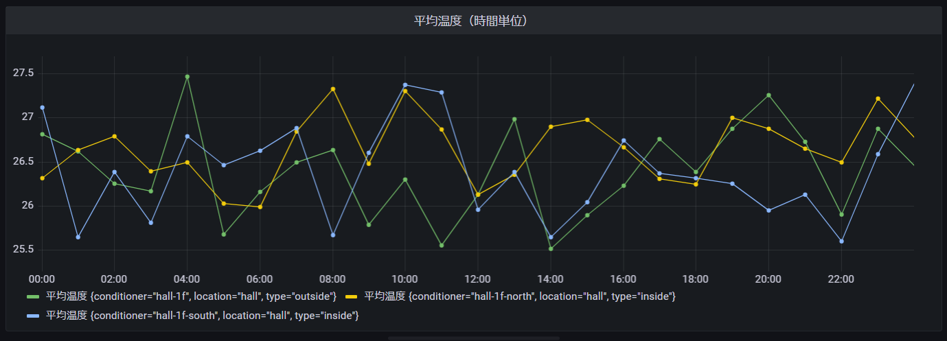
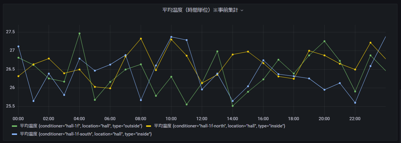
平均温度(時間単位)
空調(エアコン)毎の1時間単位の平均温度です。
WITH区で温度の1時間平均を取得し、「CREATE_TIME_SERIES」関数にて時系列モデルに変換しております。
クエリ
--AVG Temperature Per Hour
WITH binned_timeseries AS (
    SELECT location,type,conditioner, BIN(time, 1h) AS binned_timestamp, ROUND(AVG(measure_value::double), 2) AS avg_current_temperature
    FROM "coe-conditioner-db"."coe-conditioner-table"
    WHERE measure_name = 'current_temperature'
        AND time > ago(30d)
    GROUP BY location,type,conditioner, BIN(time, 1h)
    ORDER BY binned_timestamp asc
)
SELECT location,type,conditioner,CREATE_TIME_SERIES(binned_timestamp, avg_current_temperature) as "平均温度"
FROM binned_timeseries
GROUP BY location,type,conditioner
ORDER BY conditioner
Grafanaダッシュボード
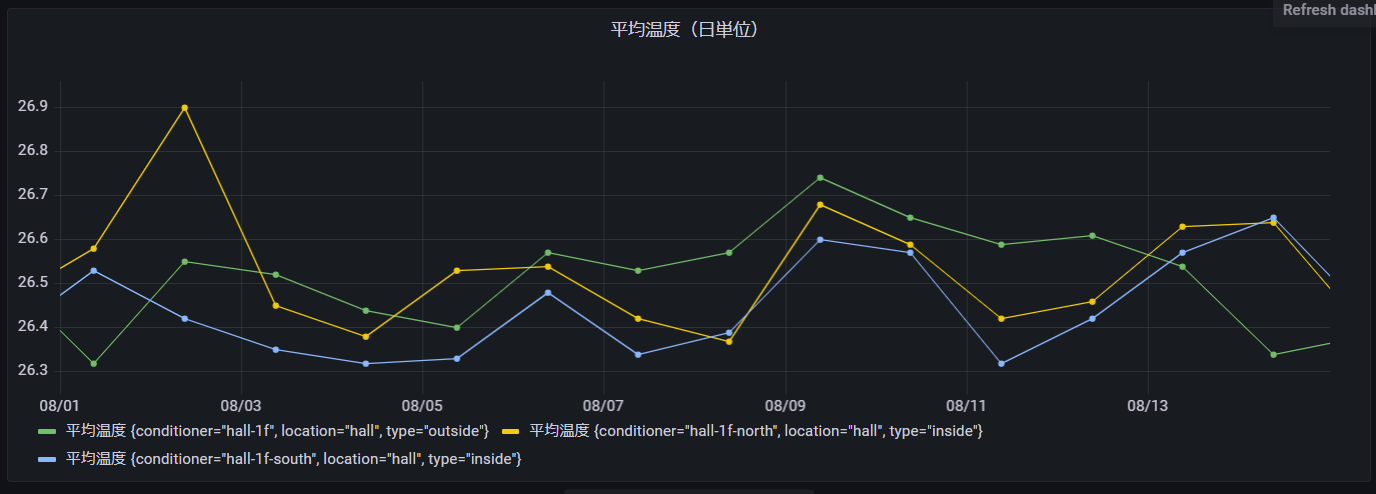
平均温度(日単位)
次に平均温度を日単位に変換して表示させてみます。WITH区の集計を時間単位から日単位に変更することで実現できます。※BIN(time, 1h) → BIN(time, 1d)
クエリ
--AVG Temperature Per Day
WITH binned_timeseries AS (
    SELECT location,type,conditioner, BIN(time, 1d) AS binned_timestamp, ROUND(AVG(measure_value::double), 2) AS avg_current_temperature
    FROM "coe-conditioner-db"."coe-conditioner-table"
    WHERE measure_name = 'current_temperature'
      AND time > ago(30d)
GROUP BY location,type,conditioner, BIN(time, 1d)
ORDER BY binned_timestamp asc
    )
SELECT location,type,conditioner,CREATE_TIME_SERIES(binned_timestamp, avg_current_temperature) as "平均温度"
FROM binned_timeseries
GROUP BY location,type,conditioner
ORDER BY conditioner
Grafanaダッシュボード
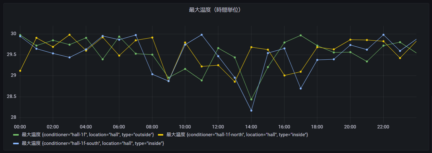
最大温度(時間単位)
次に時間単位の最大温度を表示させてみます。WITH区のAVG(平均)関数をMAX(最大)関数に変更することで実現できます。※ROUND(AVG(measure_value::double), 2) → ROUND(MAX(measure_value::double), 2)
クエリ
--MAX Temperature Per Hour
WITH binned_timeseries AS (
    SELECT location,type,conditioner, BIN(time, 1h) AS binned_timestamp, ROUND(MAX(measure_value::double), 2) AS max_current_temperature
    FROM "coe-conditioner-db"."coe-conditioner-table"
    WHERE measure_name = 'current_temperature'
      AND time > ago(30d)
GROUP BY location,type,conditioner, BIN(time, 1h)
ORDER BY binned_timestamp asc
    )
SELECT location,type,conditioner,CREATE_TIME_SERIES(binned_timestamp, max_current_temperature) as "最大温度"
FROM binned_timeseries
GROUP BY location,type,conditioner
ORDER BY conditioner
Grafanaダッシュボード
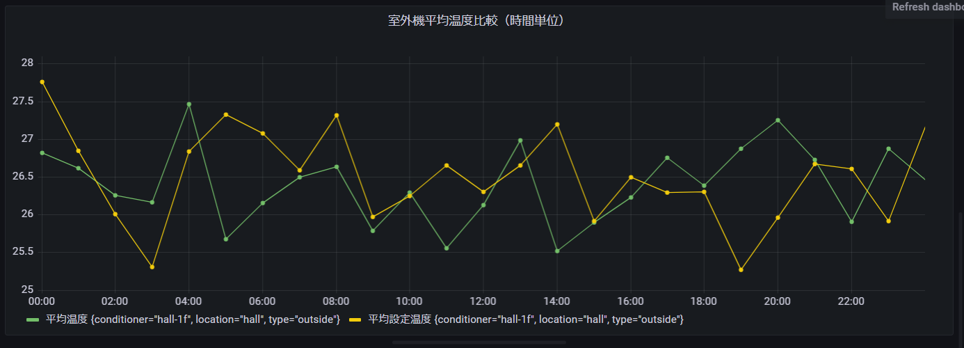
温度比較(時間単位) 1F室外機
次に実際の温度と設定温度の比較をしてみたいと思います。
Grafanaの場合は、クエリ記述エリアに2つのクエリを個々に記述してしまえば認識してくれます。
もし、1クエリで記述したい場合は、フラットに結合する以下のようなクエリを書くことができます。
クエリ
WITH binned_timeseries_current AS (
    SELECT location,type,conditioner, BIN(time, 1h) AS binned_timestamp, ROUND(AVG(measure_value::double), 2) AS avg_current_temperature
    FROM "coe-conditioner-db"."coe-conditioner-table"
    WHERE measure_name = 'current_temperature'
        AND conditioner = 'hall-1f'
        AND time > ago(30d)
    GROUP BY location,type,conditioner, BIN(time, 1h)
    ORDER BY binned_timestamp asc
),binned_timeseries_setting AS (
    SELECT location,type,conditioner, BIN(time, 1h) AS binned_timestamp, ROUND(AVG(measure_value::double), 2) AS avg_setting_temperature
    FROM "coe-conditioner-db"."coe-conditioner-table"
    WHERE measure_name = 'setting_temperature'
        AND conditioner = 'hall-1f'
        AND time > ago(30d)
    GROUP BY location,type,conditioner, BIN(time, 1h)
    ORDER BY binned_timestamp asc
)
SELECT current.location,current.type,current.conditioner,current.avg as "平均温度", setting.avg as "平均設定温度" FROM
(
  SELECT location,type,conditioner,CREATE_TIME_SERIES(binned_timestamp, avg_current_temperature) as avg
  FROM binned_timeseries_current
  GROUP BY location,type,conditioner
  ORDER BY conditioner
) current,
(
  SELECT location,type,conditioner,CREATE_TIME_SERIES(binned_timestamp, avg_setting_temperature) as avg
  FROM binned_timeseries_setting
  GROUP BY location,type,conditioner
  ORDER BY conditioner
)setting
Grafanaダッシュボード
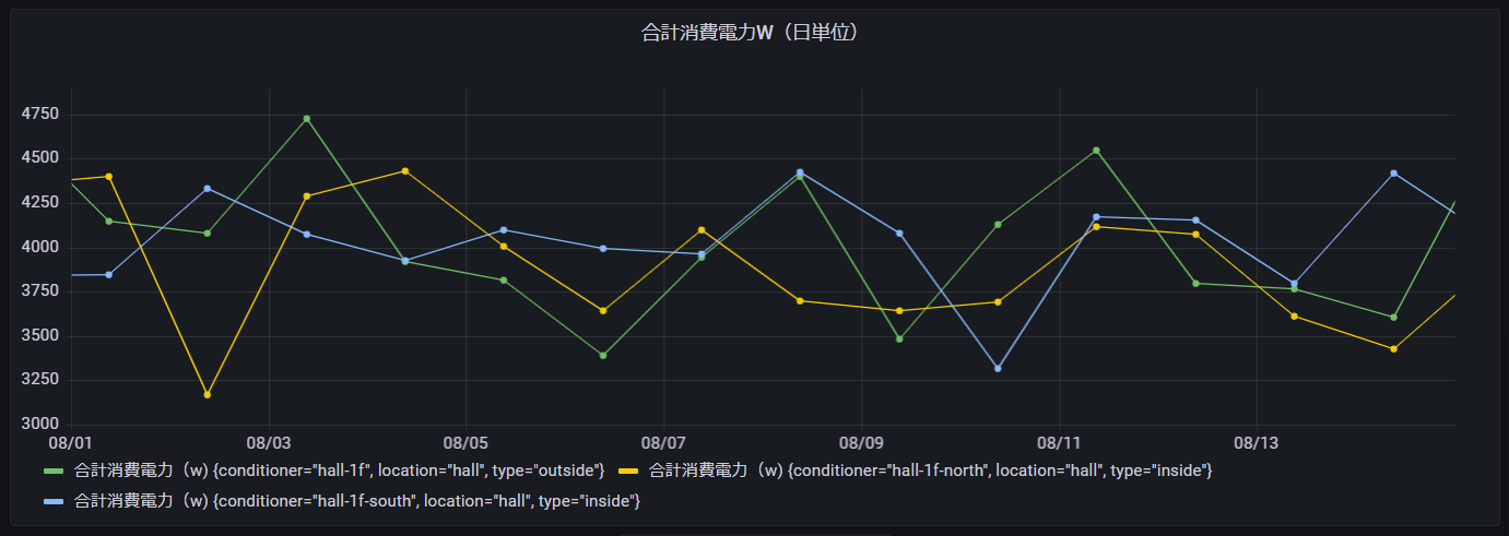
合計消費電力(日単位)
今度は60分単位の累積値である消費電力について、日単位の合計消費電力を表示させてみます。SUM(合計)関数を使用して集計することで実現できます。
クエリ
--SUM PowerConsumption Per Hour
WITH binned_timeseries AS (
    SELECT location,type,conditioner, BIN(time, 1d) AS binned_timestamp, ROUND(SUM(measure_value::double), 2) AS sum_power_consumption
    FROM "coe-conditioner-db"."coe-conditioner-table"
    WHERE measure_name = 'power_consumption'
      AND time > ago(30d)
GROUP BY location,type,conditioner, BIN(time, 1d)
ORDER BY binned_timestamp asc
    )
SELECT location,type,conditioner,CREATE_TIME_SERIES(binned_timestamp, sum_power_consumption) as "合計消費電力(w)"
FROM binned_timeseries
GROUP BY location,type,conditioner
ORDER BY conditioner
Grafanaダッシュボード
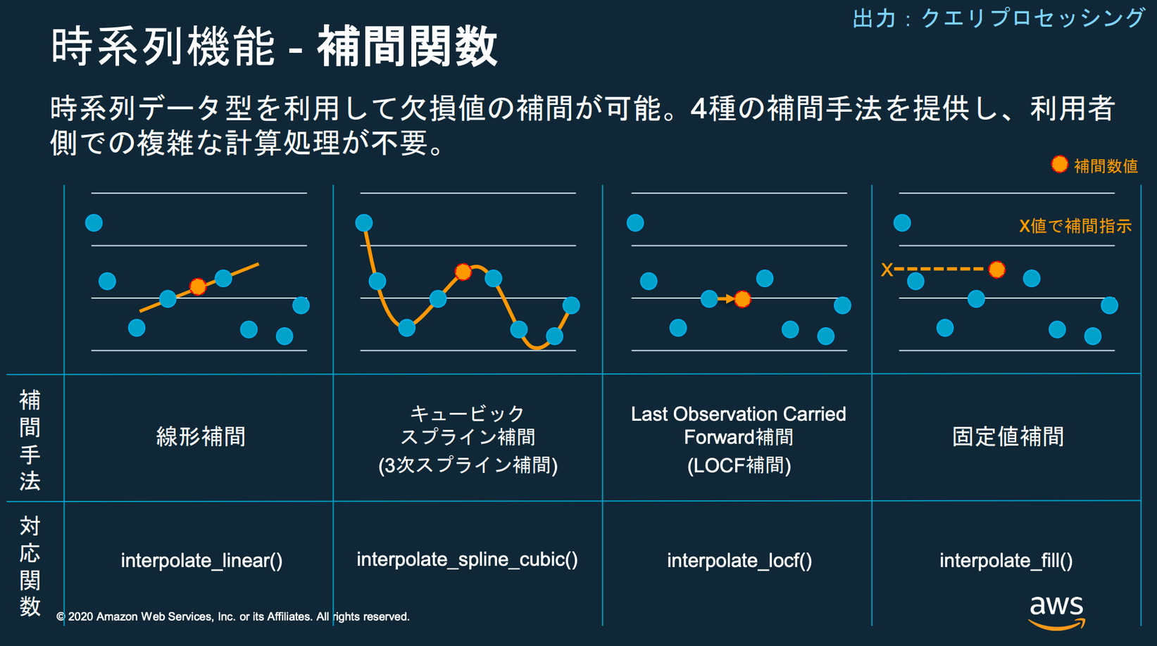
補間関数
Timestreamを利用するメリットとして、補間関数があります。
Interpolation functions – Amazon Timestream
これは集計したデータ間隔より狭い範囲で欠損した値を補間してくれる機能です。例えば、空調(エアコン)の温度データは5分間隔です。これを1分単位で集計したい場合などにTimestreamが欠損値を補間してくれます。
平均温度(1分単位) 1F室外機
補間関数の「線形補間」を利用して、空調(エアコン)の平均温度を1分単位で表示させてみます。
5分単位の温度データを「INTERPOLATE_LINEAR」関数により1分単位データとして補間します。
クエリ
WITH binned_timeseries AS (
SELECT location,type,conditioner, BIN(time, 5m) AS binned_timestamp, ROUND(measure_value::double, 2) AS avg_current_temperature
FROM "coe-conditioner-db"."coe-conditioner-table"
WHERE measure_name = 'current_temperature'
    AND conditioner = 'hall-1f'
    AND time > ago(2d)
GROUP BY location,type,conditioner, BIN(time, 5m),ROUND(measure_value::double, 2)
), interpolated_timeseries AS (
SELECT location,type,conditioner,
    INTERPOLATE_LINEAR(
        CREATE_TIME_SERIES(binned_timestamp, avg_current_temperature),
            SEQUENCE(min(binned_timestamp), max(binned_timestamp), 1m)) AS interpolated_avg_current_temperature
FROM binned_timeseries
GROUP BY location,type,conditioner
)
SELECT time, ROUND(value, 2) AS "ホール1F 室外機"
FROM interpolated_timeseries
CROSS JOIN UNNEST(interpolated_avg_current_temperature)
Grafanaダッシュボード
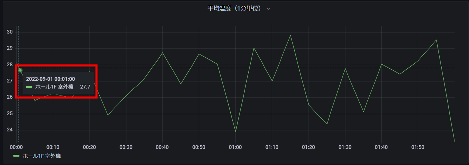
上記の通り、5分間隔のデータにも関わらず、補間関数により1分単位のデータポイントで集計・表示することが可能です。
フラットモデル
ここまで時系列モデルベースのクエリを実装して試してみましたが、Timestreamは通常のRDBMSのクエリのようにフラットモデルも利用することができます。
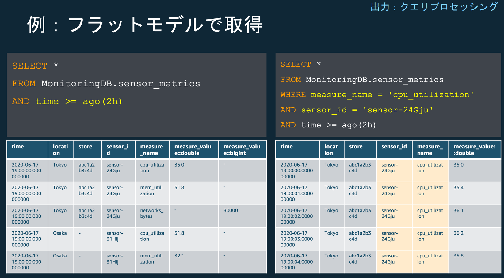
例えば、消費電力合計を週単位や月単位で集計したい場合、筆者の知る限りそれらの単位で集計する関数は用意されていません。(最大が日単位での集計)
そのような要件があった場合は以下のようにフラットモデルで取得する必要があると思っています。
合計消費電力(週単位)
クエリ
--SUM PowerConsumption Per Week (using Flat Model)
SELECT location,type,conditioner, week(BIN(time, 1d)) AS week, ROUND(SUM(measure_value::double), 2) AS "合計消費電力(w)"
FROM "coe-conditioner-db"."coe-conditioner-table"
WHERE measure_name = 'power_consumption'
  AND time > ago(365d)
GROUP BY location,type,conditioner, week(BIN(time, 1d))
ORDER BY week,conditioner
結果レコード
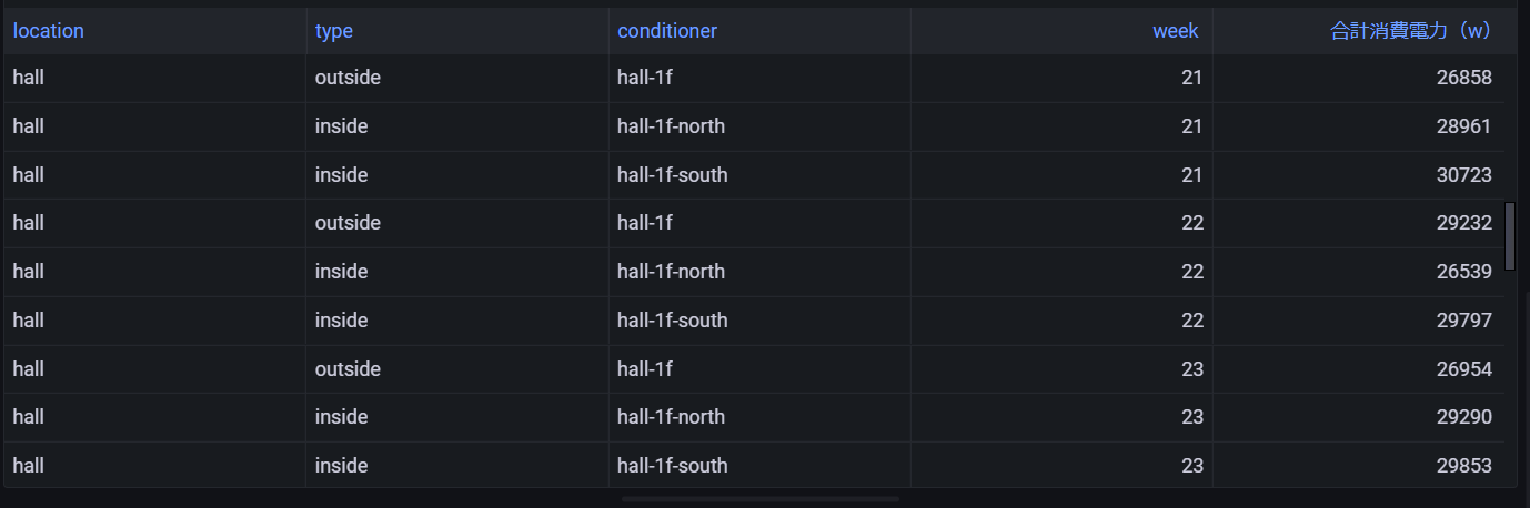
※1年の中の「何週目」として取得
合計消費電力(月単位)
クエリ
--SUM PowerCnsumption Per Month (using Flat Model)
SELECT location,type,conditioner, month(BIN(time, 1d)) AS month, ROUND(SUM(measure_value::double), 2) AS "合計消費電力(w)"
FROM "coe-conditioner-db"."coe-conditioner-table"
WHERE measure_name = 'power_consumption'
  AND time > ago(365d)
GROUP BY location,type,conditioner, month(BIN(time, 1d))
ORDER BY month,conditioner
結果レコード
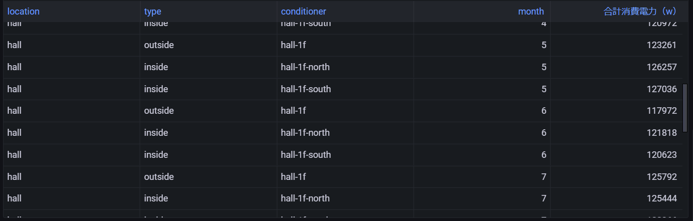
※1年の中の「何ヶ月目」として取得
また、「特定期間を通してのメトリクスを任意の単位で集計したい」ような要件もあるかと思います。このような場合も時系列モデルへの変換が難しく、以下のようにフラットモデルでの取得になると思います。
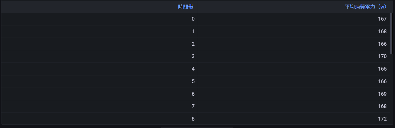
年間の時間帯毎の平均消費電力
クエリ
--AVG PowerConsumption By hour Of the year(using Flat Model)
select hour(binned_time) as "時間帯", avg(avg_power_consumption) as "平均消費電力(w)" from (
    select bin(time, 1h) as binned_time, ROUND(avg("measure_value::double"), 2) as avg_power_consumption from "coe-conditioner-db"."coe-conditioner-table"
    where measure_name = 'power_consumption'
    and time > ago(365d)
    group by bin(time, 1h)
    )
group by hour(binned_time)
order by "時間帯"
結果レコード
以上のように、時系列モデル、フラットモデルどちらを利用して可視化するかは、要件に応じて選択していくことになると思います。
スケジュールドクエリ
Timestreamには、「スケジュールドクエリ」機能があり、事前に集計したいデータに対してスケジュール化したクエリを実行し、集計結果を別テーブルに保存しておくことができます。
Using scheduled queries in Timestream – Amazon Timestream
これを利用すると以下のようなメリットが生まれます。
- クエリ実行対象のテーブルを事前集計テーブルにすることにより、クエリ実行時に毎回集計する必要がなくなり、クエリ実行速度を高めることができる
- クエリの実装が非常にシンプルになる
- クエリ実行時のスキャンバイト数が減る為、コスト効率が良くなる
- CumulativeBytesScanned:クエリによってスキャンされたバイト数
- CumulativeBytesMetered:クエリで計測された請求対象のバイト数
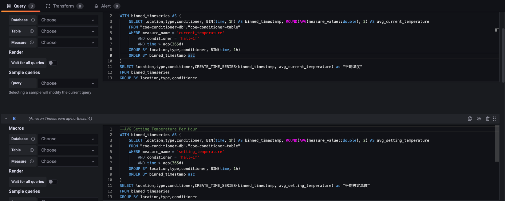
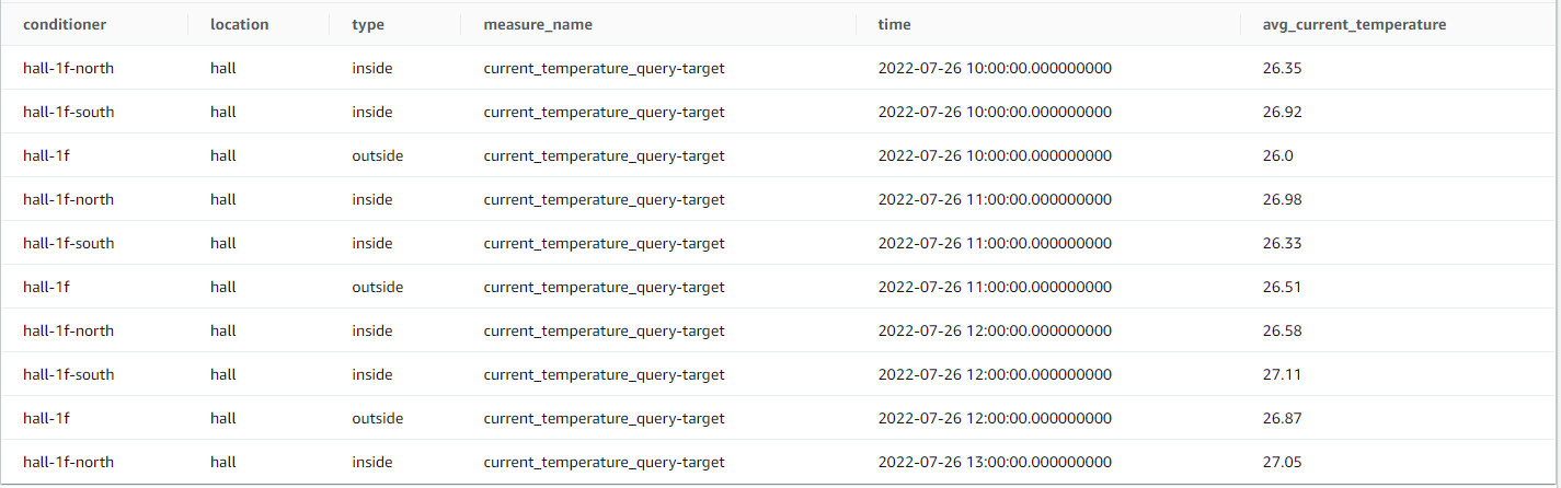
先で可視化した「平均温度(時間単位)」について、スケジュールドクエリを使用した場合にどの程度の差が出るのか比較してみました。
以下のような事前に温度平均で集計するスケジュールドクエリを定義します。
![]()
上記スケジュールドクエリを実行し、結果を別テーブルに保存しておきます。
事前集計テーブルを利用したクエリは以下のようにシンプルなものになります。
クエリ
SELECT
 location,
 type,
 conditioner,
 CREATE_TIME_SERIES(time, avg_current_temperature) as "平均温度"
FROM
 "coe-conditioner-db"."coe-conditioner-table-scheduled"
WHERE
 time > ago(30d)
GROUP BY location,type,conditioner
ORDER BY conditioner
結果は先で可視化した「平均温度(時間単位)」と同様になることが確認できます。
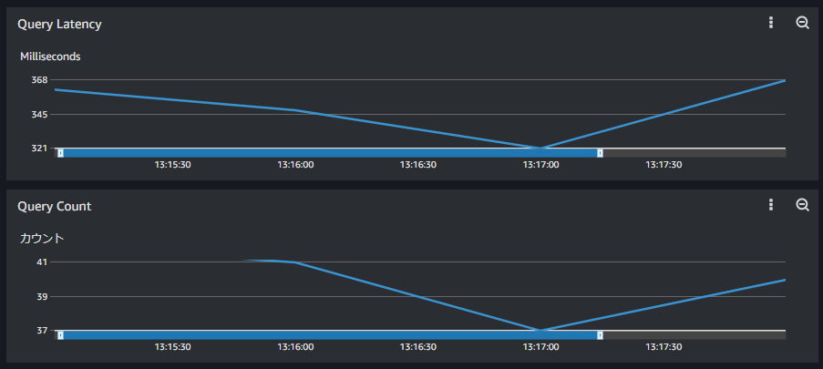
クエリ実行速度比較
では、通常(クエリ内で集計)のクエリと事前集計済みテーブルを参照したクエリの実行速度を比較してみます。
通常版
事前集計済み版
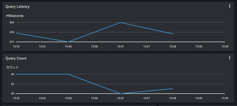
通常クエリが平均300ms台なのに対して、事前集計済みクエリは200ms台で処理できています。やはり速度的にもアドバンテージがあることが確認できました。
スキャンバイト数
次にスキャンバイト数の比較です。
以下のページのコードでクエリステータスにアクセスすることで、スキャンバイト数と請求対象のバイト数を出力することができます。
Run query – Amazon Timestream
実行結果
#通常版のクエリ
2022-09-02 19:18:19.352 [main] INFO CoeSingleMeasureClient  - query->WITH binned_timeseries AS (
    SELECT location,type,conditioner, BIN(time, 1h) AS binned_timestamp, ROUND(AVG(measure_value::double), 2) AS avg_current_temperature
    FROM "coe-conditioner-db"."coe-conditioner-table"
    WHERE measure_name = 'current_temperature'
        AND time > ago(30d)
    GROUP BY location,type,conditioner, BIN(time, 1h)
    ORDER BY binned_timestamp asc
)
SELECT location,type,conditioner,CREATE_TIME_SERIES(binned_timestamp, avg_current_temperature) as "平均温度"
FROM binned_timeseries
GROUP BY location,type,conditioner
ORDER BY conditioner ASC (CoeSingleMeasureClient.java:208)
2022-09-02 19:18:20.702 [main] INFO CoeSingleMeasureClient  - Query progress so far: 100.0% (CoeSingleMeasureClient.java:221)
2022-09-02 19:18:20.703 [main] INFO CoeSingleMeasureClient  - Bytes scanned so far: 0.001093834638595581 GB (CoeSingleMeasureClient.java:224)
2022-09-02 19:18:20.704 [main] INFO CoeSingleMeasureClient  - Bytes metered so far: 0.009313225746154785 GB (CoeSingleMeasureClient.java:227)
2022-09-02 19:18:20.705 [main] INFO CoeSingleMeasureClient  - Metadata: [ColumnInfo(Name=location, Type=Type(ScalarType=VARCHAR)), ColumnInfo(Name=type, Type=Type(ScalarType=VARCHAR)), ColumnInfo(Name=conditioner, Type=Type(ScalarType=VARCHAR)), ColumnInfo(Name=平均温度, Type=Type(TimeSeriesMeasureValueColumnInfo=ColumnInfo(Type=Type(ScalarType=DOUBLE))))] (CoeSingleMeasureClient.java:232)

#事前集計版
2022-09-02 19:18:20.734 [main] INFO CoeSingleMeasureClient  - query->SELECT
 location,
 type,
 conditioner,
 CREATE_TIME_SERIES(time, avg_current_temperature) as "平均温度"
FROM
 "coe-conditioner-db"."coe-conditioner-table-scheduled"
WHERE
 time > ago(30d)
GROUP BY location,type,conditioner
ORDER BY conditioner
 (CoeSingleMeasureClient.java:208)
2022-09-02 19:18:21.067 [main] INFO CoeSingleMeasureClient  - Query progress so far: 100.0% (CoeSingleMeasureClient.java:221)
2022-09-02 19:18:21.068 [main] INFO CoeSingleMeasureClient  - Bytes scanned so far: 9.106844663619995E-5 GB (CoeSingleMeasureClient.java:224)
2022-09-02 19:18:21.068 [main] INFO CoeSingleMeasureClient  - Bytes metered so far: 0.009313225746154785 GB (CoeSingleMeasureClient.java:227)
2022-09-02 19:18:21.068 [main] INFO CoeSingleMeasureClient  - Metadata: [ColumnInfo(Name=location, Type=Type(ScalarType=VARCHAR)), ColumnInfo(Name=type, Type=Type(ScalarType=VARCHAR)), ColumnInfo(Name=conditioner, Type=Type(ScalarType=VARCHAR)), ColumnInfo(Name=平均温度, Type=Type(TimeSeriesMeasureValueColumnInfo=ColumnInfo(Type=Type(ScalarType=DOUBLE))))] (CoeSingleMeasureClient.java:232)
通常版のクエリの「CumulativeBytesScanned(クエリによってスキャンされたバイト数)」が「0.001093834638595581GB→およそ1.09MB」に対して、事前集計版は「9.106844663619995E-5 GB→およそ0.09MB」と、1/10以上の効果がありました。
※CumulativeBytesMetered(クエリで計測された請求対象のバイト数)がおよそ10MB、かつ両者に差異がないのは、請求の対象の最小値が「10MB」なので、それに丸められている為です。
(再掲)Amazon Timestream pricing より
クエリ: Amazon Timestream のサーバーレス分散型クエリエンジンがクエリ結果を計算する際にスキャンしたデータ量 (最も近い MB に丸められ、最小値は 10 MB です)
さいごに
時系列DBには「InfluxDB」や「Timescale」などありますが、運用管理を考えると導入のハードルが高いと思っていました。Timestreamは検証結果からもわかる通り、構築も容易で、サーバを管理する必要もない為、そのハードルは非常に低いと感じました。また、コスト的にも低コストで大量のストリームデータを処理できる為、データ分析・予測のユースケースで大きな力を発揮するサービスだと思います。
本記事にて検証内容を共有させていただきましたが、準備することもほとんどなく、すぐに試すことが出来ますので、是非一度触ってみていただければと思います。
以上